Building a portfolio optimizer in 100 Lines of Code

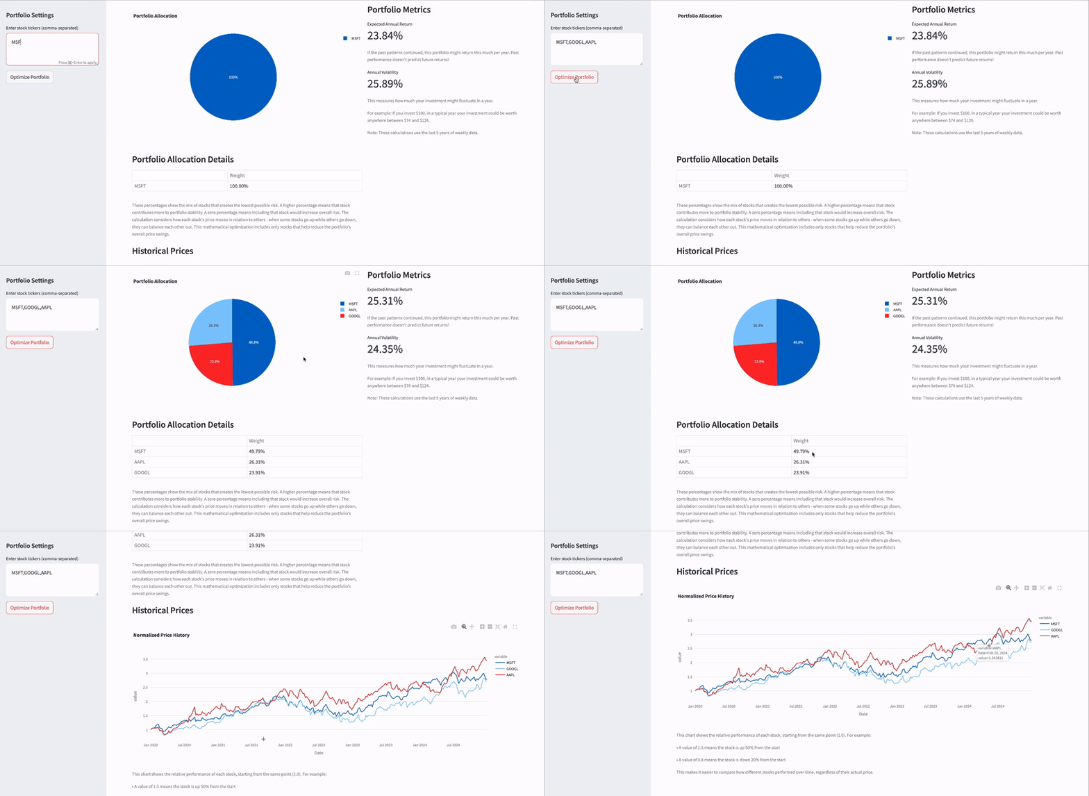
Here's the tool in action, showing how you can quickly analyze different stock combinations.
Try it yourself: https://portfolio-optimization-demo.streamlit.app/
⚠️ This is an educational project to demonstrate rapid prototyping with Streamlit. This is not financial advice. Use of this tool is at your own risk. The creators and contributors of this project are not responsible for any financial losses or decisions made based on this tool. Past performance does not guarantee future results. Always consult with qualified financial professionals before making investment decisions.
Quick Start Guide
- Visit the live demo
- Enter stock tickers in the sidebar (e.g., "AAPL,MSFT,GOOGL") or simply use the default
- Click "Optimize Portfolio" to see the recommended allocation
- The pie chart shows the optimal mix of stocks for minimum risk
- Check the metrics on the right for expected return and volatility
1. Getting Stock Data
The first challenge is getting reliable stock data. I use yfinance because it's free and easy to use. Here's how I fetch and clean the data:
def load_stock_data(tickers, period="5y", interval="1wk"):
    df = pd.DataFrame()
    failed_tickers = []

    if isinstance(tickers, str):
        tickers = [ticker.strip().upper() for ticker in tickers.split(',')]

    for ticker in tickers:
        try:
            data = yf.download(ticker, period=period, interval=interval, progress=False)
            if not data.empty:
                df[ticker] = data['Adj Close']
        except Exception as e:
            failed_tickers.append(ticker)

    return df.ffill().dropna()
Let's break down what's happening here:
- We download historical stock prices directly from Yahoo Finance using the yfinance library
- The data covers 5 years of weekly price movements for better analysis
- Built-in error handling ensures the code continues running even with invalid tickers
- Missing data points are handled through forward-fill, and any remaining gaps are removed
- We use adjusted closing prices to account for stock splits and dividend payments
2. Portfolio Analysis
This section handles the portfolio optimization using Modern Portfolio Theory to find the lowest-risk combination of stocks. For this I use the PyPortfolioOpt library, which features Python implementation of various portfolio optimization techniques and in my opinion is the best library for this purpose.
def optimize_portfolio(prices):
    returns = prices.pct_change().dropna()
    weekly_vol = returns.std()
    annual_vol = weekly_vol * np.sqrt(52)

    S = returns.cov() * 52  # Annualized covariance
    mu = returns.mean() * 52  # Annualized returns

    ef = EfficientFrontier(mu, S)
    weights = ef.min_volatility()
    cleaned_weights = ef.clean_weights()

    expected_return, volatility, sharpe = ef.portfolio_performance()
    return cleaned_weights, expected_return, volatility, sharpe
The code converts price data into returns and annualizes the numbers by multiplying by √52. This √52 factor comes from the statistical property of volatility scaling with the square root of time - since there are 52 weeks in a year, we multiply weekly volatility by √52 to get annual volatility. This same principle applies when converting weekly returns to annual returns, where we multiply by 52 (not the square root) because returns add linearly over time.
PyPortfolioOpt handles the heavy lifting of finding the optimal weights. The optimization results tell an important story: stocks with higher weights are those that contribute most to portfolio stability, while those with zero or near-zero weights would likely increase overall risk. This works because the algorithm considers how stocks move in relation to each other - when some go up while others go down, they can help balance each other out, reducing the portfolio's overall volatility.
3. Visualization with Streamlit
Finally, I create an interactive interface that makes this analysis accessible to anyone:
# Input section
with st.sidebar:
    ticker_input = st.text_area("Enter stock tickers", "MSFT,GOOGL,AMZN,AAPL")
    if st.button("Optimize Portfolio"):
        prices = load_stock_data(ticker_input.split(","))
        weights, exp_return, vol, sharpe = optimize_portfolio(prices)

# Results visualization
st.info("These percentages show the mix of stocks that creates the lowest possible risk. A higher percentage means that stock contributes more to portfolio stability.")

col1, col2 = st.columns([3, 2])
with col1:
    # Portfolio allocation pie chart
    fig = px.pie(weights_df,
                 values='Weight',
                 names=weights_df.index,
                 title='Portfolio Allocation')
    st.plotly_chart(fig)

with col2:
    # Key metrics
    st.metric("Expected Return", f"{exp_return:.2%}")
    st.metric("Volatility", f"{vol:.2%}")
The visualization layer does several important things:
- A clean sidebar interface lets users type in their stock picks and instantly see results
- The pie chart gives a visual understanding of how investments are devided according to the results of the optimization method
- Clear percentage breakdowns show both potential gains and risks at a glance
- The two-column layout keeps everything organized without overwhelming the user
What makes this special is how Streamlit handles all the web development complexity. We don't need to write any HTML, CSS, or JavaScript - it's all pure Python.

Here's the tool in action, showing how you can quickly analyze different stock combinations.
The entire application comes together in less than 120 lines of code, demonstrating how modern Python libraries let us build sophisticated tools quickly. While this is a simplified version of portfolio optimization, it shows the core concepts and could be extended with more advanced features like:
- More sophisticated optimization strategies beyond minimum volatility
- Advanced risk metrics that consider market conditions
- Historical performance testing to validate strategies
- Smart rebalancing recommendations based on market changes
Complete Code
Here's the working code for the portfolio optimizer reduced to its essentials. You can copy this into a file named app.py and run it with streamlit run app.py:
import streamlit as st
import yfinance as yf
import numpy as np
import pandas as pd
from pypfopt import EfficientFrontier, risk_models, expected_returns
import plotly.express as px

st.set_page_config(page_title="Portfolio Optimizer", layout="wide")

def load_stock_data(tickers, period="5y", interval="1wk"):
    df = pd.DataFrame()
    failed_tickers = []

    if isinstance(tickers, str):
        tickers = [ticker.strip().upper() for ticker in tickers.split(',')]
    else:
        tickers = [ticker.strip().upper() for ticker in tickers]

    for ticker in tickers:
        try:
            data = yf.download(ticker, period=period, interval=interval, progress=False)
            if data.empty:
                failed_tickers.append(ticker)
                continue
            if 'Adj Close' in data.columns:
                df[ticker] = data['Adj Close']
            else:
                df[ticker] = data['Close']

        except Exception as e:
            failed_tickers.append(ticker)
            st.error(f"Error loading data for {ticker}: {str(e)}")
            continue
    if df.empty:
        raise ValueError("No data was loaded. Please check your ticker symbols.")
    if failed_tickers:
        st.warning(f"Failed to load data for: {', '.join(failed_tickers)}")
    df = df.ffill().dropna()
    return df

def optimize_portfolio(prices):
    returns = prices.pct_change().dropna()
    weekly_vol = returns.std()
    annual_vol = weekly_vol * np.sqrt(52)
    S = returns.cov() * 52
    mu = returns.mean() * 52

    ef = EfficientFrontier(mu, S)
    weights = ef.min_volatility()
    cleaned_weights = ef.clean_weights()
    expected_return, volatility, sharpe = ef.portfolio_performance()

    return cleaned_weights, expected_return, volatility, sharpe

st.title("Minimizing portfolio risk (educational demo)")

if 'first_load' not in st.session_state:
    st.session_state.first_load = True

with st.sidebar:
    st.header("Portfolio Settings")
    ticker_input = st.text_area("Enter stock tickers (comma-separated)", "MSFT,GOOGL,AMZN,AAPL")
    if st.button("Optimize Portfolio") or st.session_state.first_load:
        st.session_state.first_load = False
        tickers = [ticker.strip() for ticker in ticker_input.split(",")]

        with st.spinner("Loading data and optimizing portfolio..."):
            try:
                prices = load_stock_data(tickers)
                weights, exp_return, vol, sharpe = optimize_portfolio(prices)

                st.session_state.weights = weights
                st.session_state.metrics = {
                    "Expected Return": exp_return,
                    "Volatility": vol,
                    "Sharpe Ratio": sharpe
                }
                st.session_state.prices = prices

            except Exception as e:
                st.error(f"An error occurred: {str(e)}")

col1, col2 = st.columns([3, 2])
with col1:
    if "weights" in st.session_state:
        weights_df = pd.DataFrame.from_dict(st.session_state.weights, orient='index', columns=['Weight'])
        weights_df['Allocation'] = weights_df['Weight'].apply(lambda x: f"{x:.2%}")
        weights_df = weights_df.sort_values('Weight', ascending=False)
        fig = px.pie(weights_df[weights_df['Weight'] > 0],
                    values='Weight',
                    names=weights_df[weights_df['Weight'] > 0].index,
                    title='Portfolio Allocation')
        st.plotly_chart(fig)

        st.subheader("Portfolio Allocation Details")
        st.table(weights_df[['Allocation']].rename(columns={'Allocation': 'Weight'}))
with col2:
    if "metrics" in st.session_state:
        st.subheader("Portfolio Metrics")
        metrics = st.session_state.metrics
        st.metric("Expected Annual Return", f"{metrics['Expected Return']:.2%}")
        st.metric("Annual Volatility", f"{metrics['Volatility']:.2%}")
if "prices" in st.session_state:
    st.subheader("Historical Prices")
    normalized_prices = st.session_state.prices / st.session_state.prices.iloc[0]
    fig = px.line(normalized_prices, title="Normalized Price History")
    st.plotly_chart(fig)
To run this code, you'll need to install the required packages:
pip install streamlit yfinance numpy pandas pypfopt plotly